Project Report
Retail Store Inventory and Demand Forecasting
1. Project Overview
1.1. Problem Definition and Goal
This project aims to predict retail-store product demand and connect the prediction results to inventory-management decisions. Demand forecasting is a multi-horizon time-series regression problem because future demand must be predicted across several days rather than only at one point in time. Accurate forecasts can reduce stockouts and excessive inventory, improving both sales opportunity and operating efficiency.
1.2. Evaluation Metrics
The project uses MAPE and RMSE as core metrics. MAPE measures relative error and is intuitive for business interpretation, while RMSE penalizes large forecast errors more strongly. Quantile forecasts are also used because demand uncertainty matters for safety-stock decisions. The target was to improve meaningfully over a baseline and approach a MAPE of around 10%.
2. Data Overview
2.1. Data Source and Structure
The dataset contains retail-store inventory and demand records. Each row includes a date, store, product, category, region, inventory level, units sold, units ordered, price, discount, weather condition, promotion status, competitor pricing, seasonality, epidemic status, and demand.
The data has the form of a panel time series because demand is observed repeatedly across multiple store-product combinations. Therefore, the model must learn both time-dependent patterns and static differences between products and stores.
The variables were defined in detail according to the TFT input structure.
- Static Covariates: properties that do not change over time, including store ID, product ID, category, and region.
- Time-varying Known Inputs: information known in advance for future time points, including date, day of week, weekend flag, seasonality, and promotion plans.
- Time-varying Unknown Inputs: information known only up to the past, including actual demand, inventory level, sales volume, competitor price, weather, and epidemic status.
2.2. Feature Description
The features in the data are as follows.
- Date: the date the data was recorded.
- Store ID: unique identifier for each store.
- Product ID: unique identifier for each product.
- Category: product category, such as electronics or clothing.
- Region: geographical region where the store is located.
- Inventory Level: quantity currently remaining in the warehouse or store.
- Units Sold: number of products actually sold on that date.
- Units Ordered: quantity ordered for replenishment.
- Price: selling price of the product.
- Discount: applied discount rate or amount.
- Weather Condition: weather on the recorded date, such as sunny or rainy.
- Promotion: whether a promotion was active.
- Competitor Pricing: price of similar products from competitors.
- Seasonality: season corresponding to the date.
- Epidemic: whether an epidemic was present.
- Demand: estimated daily demand for the product.
3. EDA
3.1. Checking Data Distributions
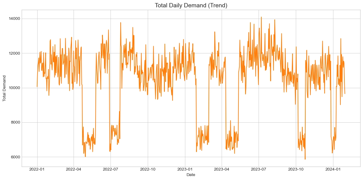
The time-series trend of daily total demand shows clear seasonality and cyclicality rather than random distribution. The decisive feature is that demand repeatedly increases and decreases over time. This confirms that the task should be approached as a time-series forecasting problem rather than a simple independent regression problem.
Because demand changes according to temporal conditions, the model needs date-derived features such as day of week, weekend flag, and season.
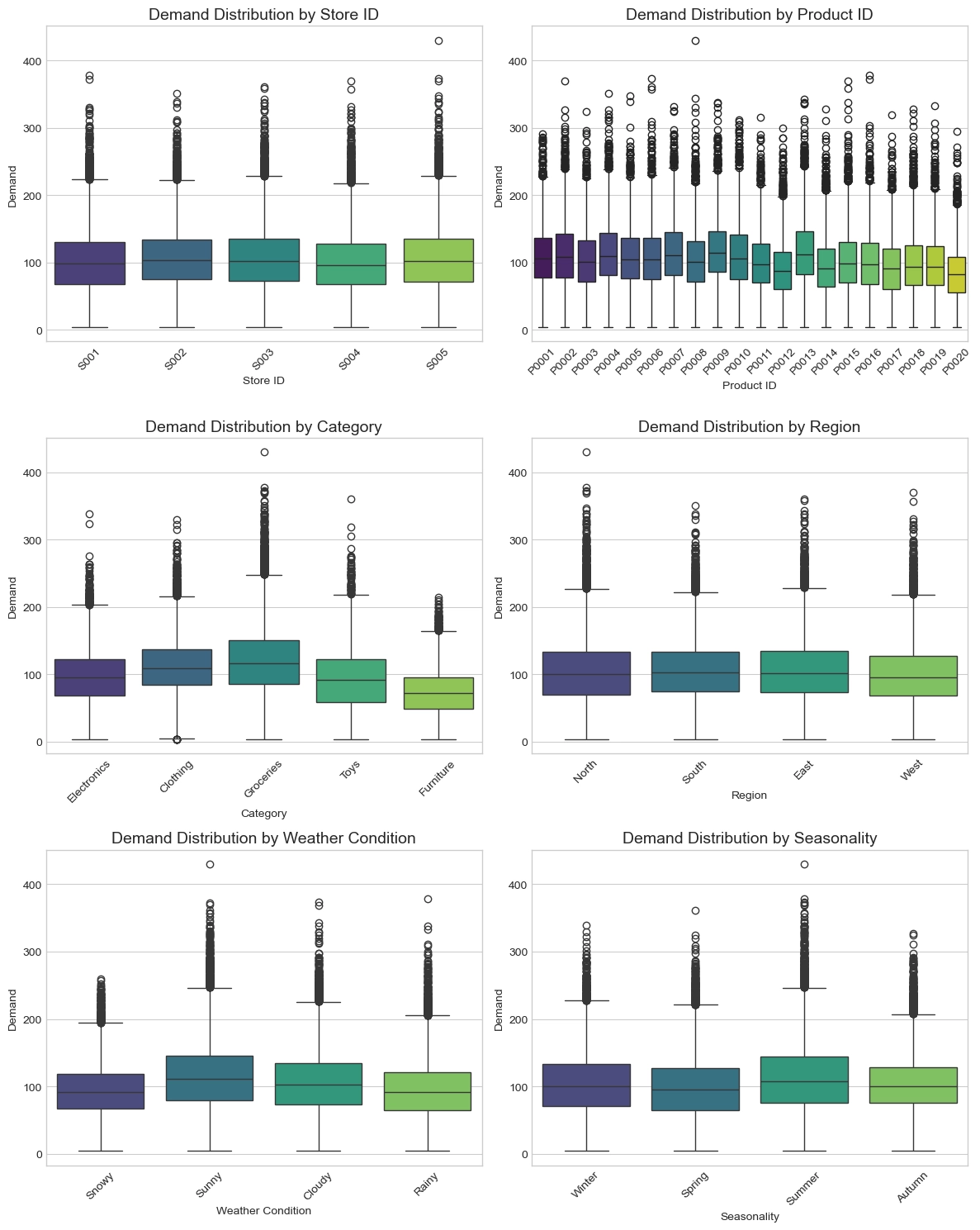
Demand distribution by categorical feature shows that product category and weather condition strongly affect individual product demand. Some categories have consistently high demand, while others show lower and more volatile demand. This supports the use of category and product identifiers as static covariates.
Weather and seasonality also affect demand differences, indicating that external conditions should be included as known or observed time-varying inputs.
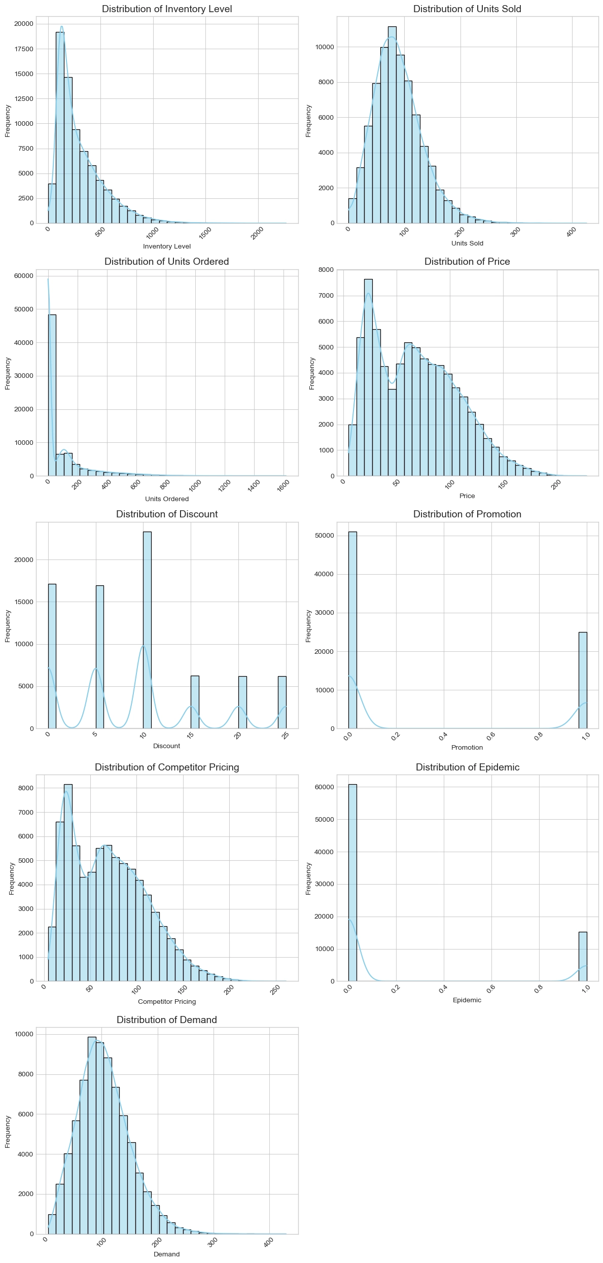
Demand and inventory-related variables show strong asymmetry. Inventory Level and Units Ordered have typical right-skewed distributions. This suggests that certain products or stores experience exceptionally high replenishment or stock levels.
3.2. Correlation and Insights
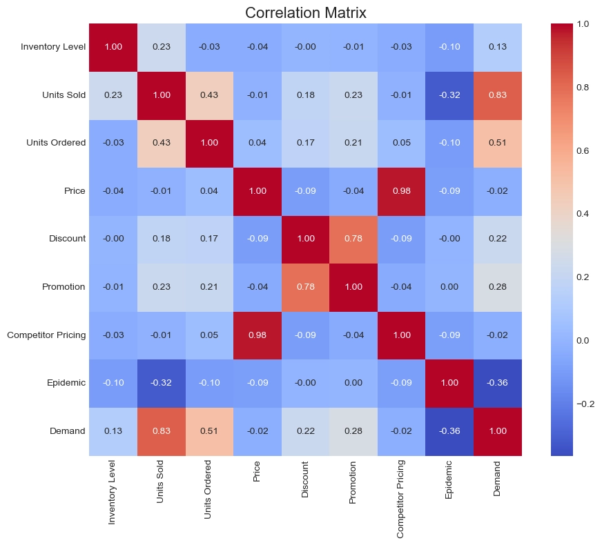
The first point to note is multicollinearity. The correlation coefficient between Price and Competitor Pricing is 0.98, meaning the two variables contain nearly identical information. If both are used without adjustment, the model may become unstable or overemphasize price-related effects.
Demand is related to Units Sold and Inventory Level, which is natural because these variables directly interact in retail operations. However, care must be taken to prevent future leakage when using variables that are unknown at prediction time.
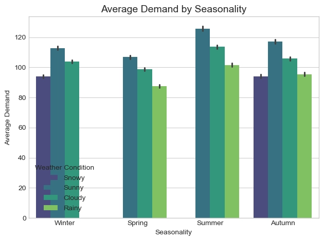
Overall, average demand is highest in summer, and demand tends to be maximized under sunny conditions in every season. In particular, the difference between sunny days and other weather conditions is large, showing that weather conditions have meaningful explanatory power.
4. Data Preprocessing
4.1. Feature Engineering
Time-related features were generated from the date column, including day of week, month, weekend flag, and season-related information. These features help the model learn recurring demand patterns and make multi-horizon prediction possible.
4.2. Preprocessing Strategy and Key Techniques
The dataset was reorganized into a sequence format appropriate for TFT. Static variables, known future variables, and unknown historical variables were separated so the model could use information in a way that matches actual forecasting conditions.
Numerical variables were scaled, categorical variables were encoded, and time indices were created for each store-product series. Missing or inconsistent records were handled before training to reduce instability.
5. Modeling and Optimization
5.1. Model Selection
The Temporal Fusion Transformer was selected because it supports multi-horizon forecasting and can use static covariates, known future variables, and observed historical variables together. Its attention mechanism also provides interpretability through variable importance.
5.2. Hyperparameter Tuning
Optuna was used for hyperparameter tuning. The search space included hidden size, dropout, hidden continuous size, attention head size, and learning rate. Garbage collection and CUDA cache cleanup were performed inside the objective function to reduce memory pressure during repeated experiments.
def objective(trial):
    gc.collect()
    torch.cuda.empty_cache()

    hidden_size = trial.suggest_categorical("hidden_size", [16, 32, 64])
    dropout = trial.suggest_float("dropout", 0.1, 0.4)
    hidden_continuous_size = trial.suggest_categorical("hidden_continuous_size", [8, 16, 32])
    attention_head_size = trial.suggest_categorical("attention_head_size", [1, 2, 4])
    learning_rate = trial.suggest_float("learning_rate", 1e-4, 1e-2, log=True)

    # build, train, validate the TFT model
    return val_loss

study.optimize(objective, n_trials=20)
5.3 Tuning Results and Best Parameters
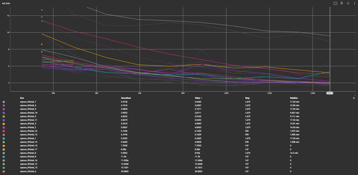
- Best trial: trial 7, value 3.6446170806884766
- Hidden Size: 64
- Learning Rate: 0.008040444263766957
- Dropout: 0.2433929223767682
- Attention Heads: 2
6. Results and Analysis
6.1. Final Performance Evaluation
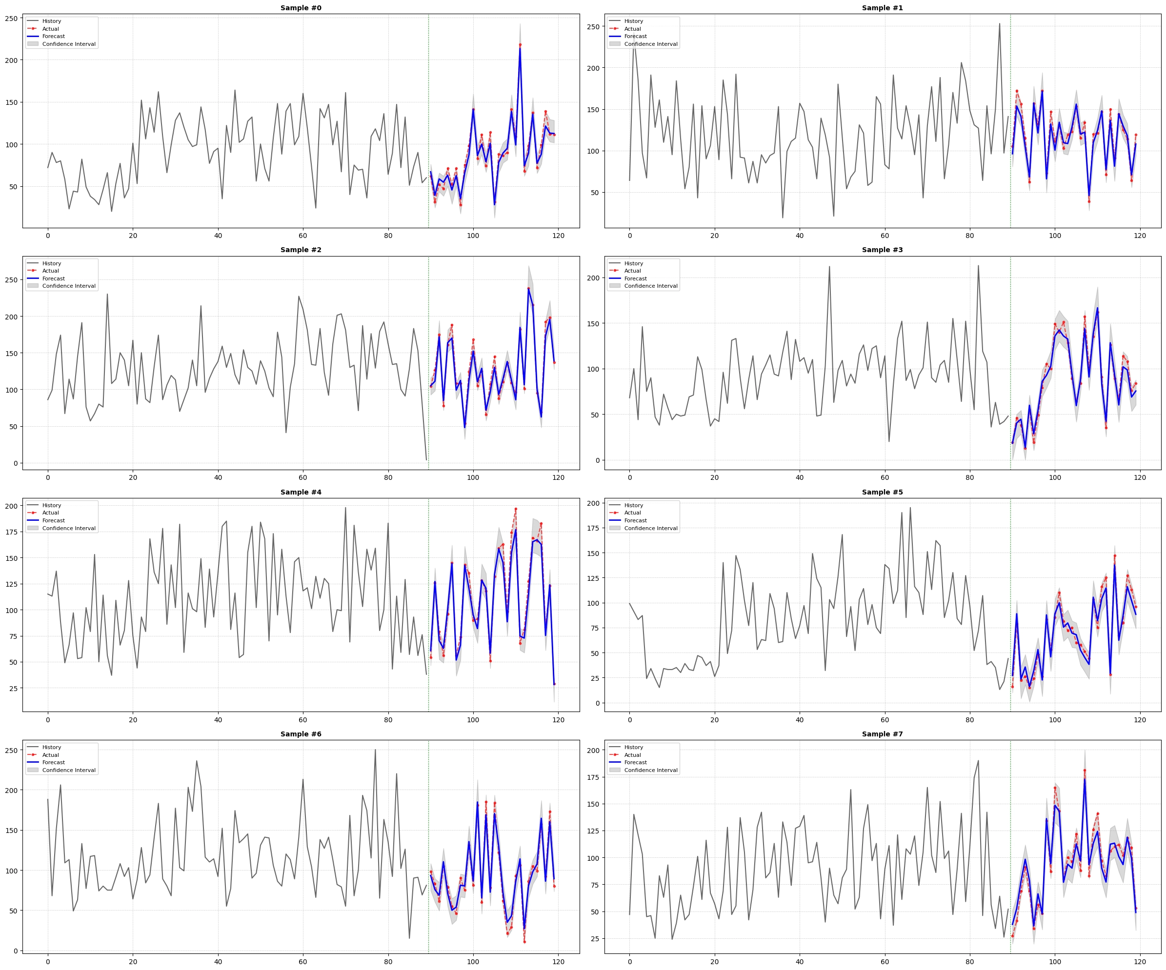
- MAPE: My Model 10.15%, Baseline 54.79%. Although it narrowly missed the target of below 10%, it improved greatly over the baseline.
- RMSE: My Model 9.14, Baseline 61.06. This is an 85.03% improvement over the baseline and sufficiently meets the goal of more than 15% improvement.
The final model substantially reduced prediction error compared with the baseline. This confirms that using a sequence model with structured covariates is effective for retail demand forecasting.
6.2. Feature Importance
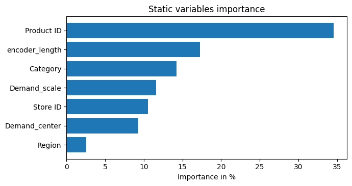
Static variable analysis shows that Product ID has the highest importance at about 35%. This means each product has a unique sales pattern, and the model relies heavily on product identity when forecasting demand.
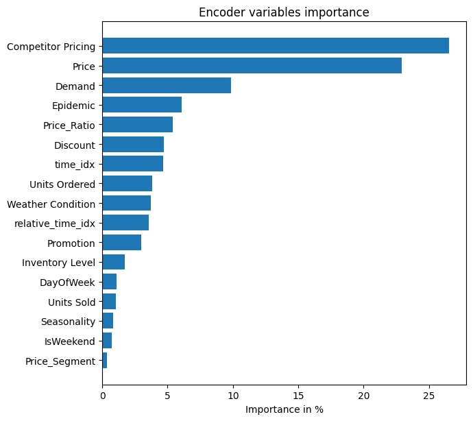
In the encoder-variable analysis, Competitor Pricing and Price together account for about 50% of importance. This indicates that the model uses price-related signals strongly when interpreting past demand patterns.
7. Conclusion
7.1. Business Impact
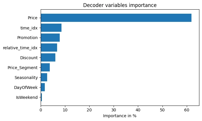
The model can support practical inventory decisions by forecasting demand more accurately than the baseline. Lower forecast error can reduce stockouts, avoid excessive ordering, and improve replenishment timing. Product-level and price-related importance also provides business insight into which factors should be monitored closely.
7.2. Limitations and Future Work
The model still narrowly misses the MAPE target of below 10%, and the dataset has limitations because some external factors are simplified. Future work includes adding richer holiday and regional event data, improving leakage control, testing additional forecasting architectures, and connecting forecasts directly to safety-stock optimization.